Excel pie chart over 100 percent

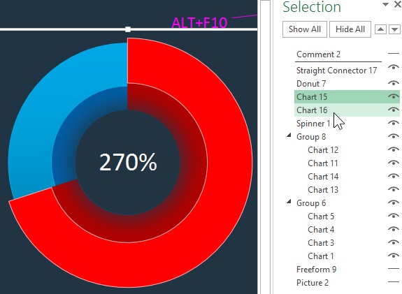
Think of it as a dial where straight up is budget rotate counterclockwise to show underbudget green wedge or rotate right to show overbudget up to 200 but the idea is extendable. The source data for the chart comes from the table above it -.

How To Make A Pie Chart In Excel

We can use the following formula to calculate the remainder value.

. Or type the number you want directly in the box. Now we have a 100 stacked chart that shows the percentage breakdown in each column. Pie Chart in Excel Pie Chart in Excel is used for showing the completion or main contribution of different segments out of 100.

The above steps would instantly add a Pie chart on your worksheet as shown below. Select the Doughnut it could be any of the pies but this is the route I took for reasons you will see. On the ribbon go to the Insert tab.

Go to the Insert tab and select the Pie Chart dropdown. This only occurs if the precision of the labels is unit percentages number format of 0 not if more precision is allowed number format of 00. In the Charts group click on the Insert Pie or Doughnut Chart icon.

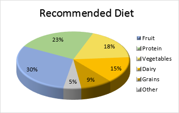
But to tell if the analysis makes sense why not tell us what analysis you did. For instance if the areas were 747 58 58 137 then normal rounding to integer percents would sum to 101 rather than 100. The categories will add up to 100 percent of whatever is being charted and the relative size of each category is a visual representation of its relation to the whole.

With a percent the percentage contribution of each type of tax in the total amount. The chart shows the percentage of income from taxation. A 100 stacked bar chart is an Excel chart type designed to show the relative percentage of multiple data series in stacked bars where the total cumulative of each stacked bar always equals 100.

100-B2 If the maximum percentage complete value can go over 100 then its best to use the following formula for the remainder value. Lets add columns to the table. I have a tee-shirt that says 2 2 5 for extremely large values of 2.

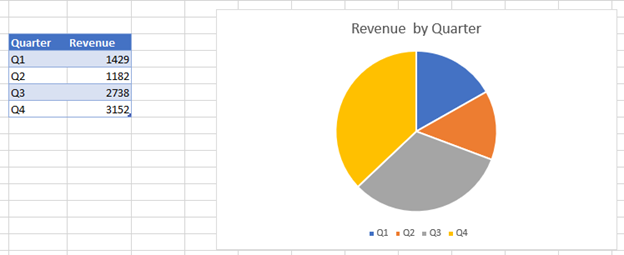
To create a pie chart highlight the data in cells A3 to B6 and follow these directions. When creating a pie chart the description of each section is called the category and the number connected to the category is called the value. Share Improve this answer answered Oct 30 2011 at 2034 Peter Flom.

A B C D etc Budget Actual C of budget BA may be larger or smaller than 100 D savings if C. Next click apply shown at the bottom-left side of the values tab. Like a pie chart a 100 stacked bar chart shows a part-to-whole relationship.

Go to the tab INSERT. MAX 100B2-B2 This will change the remainder value to zero if the progress is greater than 100. Ad Learn More About Different Chart and Graph Types With Tableaus Free Whitepaper.

To solve this problem in Excel it is best to use several charts that are superimposed on layers. If you get stuck attach your workbook and well help from there. 100 Stacked Column.

1Click Kutools Charts Category Comparison Stacked Chart with Percentage see screenshot. If desired you can pick special colors by right clicking on any data point and selecting Fill. Choose a chart type.

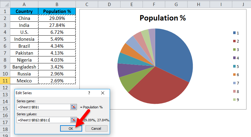
The single column column B used to create the excel pie chart is reflected under series Select or deselect the categories in order to show or hide them from the chart. Both cell values are formatted as percents. Depending on the areas of the other slices that may require at least one percentage to round in a nonstandard way.

On the Format Data Point pane under Series Options drag the Angle of first slice slider away from zero to rotate the pie clockwise. Explore Different Types of Data Visualizations and Learn Tips Tricks to Maximize Impact. Click on the Pie icon within 2-D Pie icons.

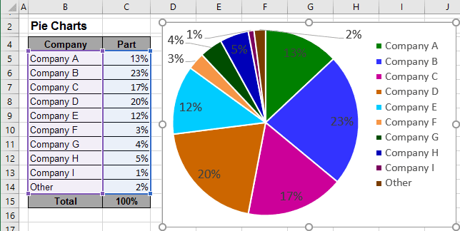
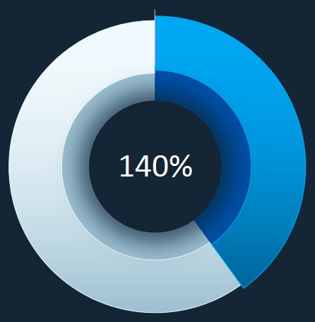
Pie chart Template for Visualizing Data Exceeding 100 The principle of building this element of the presentation is simple. Hover over a chart type to read a description of the chart and to preview the pie chart. The phenomenon is that Excel will place incorrect percentage labels onto the wedges of a pie chart simply to ensure that the displayed percentages add to 100.

In the group of Carts choose 100 Stacked. Bar Chart to Display 0 to 100 The axis values default to Auto but you can specify what they should be. To add these to the chart I need select the data labels for each series one at a time then switch to value from cells under label options.

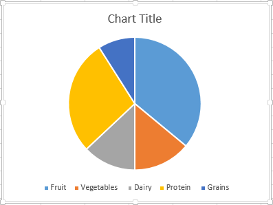
Select the entire dataset Click the Insert tab. Finally we can make the chart. It is like each value represents the portion of the Slice from the total complete Pie.

After installing Kutools for Excel please do as this. The filters will be applied to the pie chart. Pie chart with percentage is ready.

Select Insert Pie Chart to display the available pie chart types. Right-click any slice of your pie graph and click Format Data Series. Pie charts are a terrible way to visualized data.

Right click the axis numbers and select Format Axis. Excel rounds percentages on a pie chart such that they are integers that add to 100. Diagrams on each layer use their own separate source data which are composed by formulas in the range of cells A1C2.

To rotate a pie chart in Excel do the following. Select the two Helper Cells in B1 and B2. 3Then click OK button and a prompt message is.

2In the Stacked column chart with percentage dialog box specify the data range axis labels and legend series from the original data range separately see screenshot. Jun 7 2011 1 Not sure if I worded the topic title correctly but a bar chart I have created in Excel 2007 shows a maximum of 120 even though none of the source figures are more than 100. We click on any cell of the table.

For Example we have 4 values A B C and D. Ad Project Management in a Familiar Flexible Spreadsheet View. Whenever you create these kind of helper calculations for a chart take care with the Switch ColumnRow button.

Once you have the data in place below are the steps to create a Pie chart in Excel. So a limit of 0 at the bottom end and 1 at the top will equate to a 0 - 100 axis regardless of the values entered. As karl said numbers can easily add up to 101 due to rounding error.

I Will Do Statistical Graphs With Spss Excel Or R In 2022 Line Graphs Graphing Bar Chart